Commercial vehicle’s active steering srategies
Zoltán Hankovszki
PhD student
BME GJT
Roland Kovács
head of development team
Knorr-Bremse Fékrendszerek Kft.
Dr. László Palkovics
deputy head of department
BME GJT
Advanced Vehicle Control Knowledge Centre, Budapest University of Technology and Economics, HUNGARY
Abstract:
It is a timeless and actual problem to develop vehicle’s active safety [1]. In case of commercial vehicle category more sophisticated difficulties could be found. Increased mass and inertia are the fundamental differences between a usual passenger car and a truck. At the same time, the low series number requests cheap solutions. The aim is in this way to ensure low cost solutions to control increased kinetic energies.
Commercial Vehicles
As it was mentioned, increased mass and inertia are the fundamental sources of problems. To control these physical quantities special braking and steering systems are often needed [2]. Another problem is the varying of these masses and inertias. A 12tons truck’s empty weight is less than half of the laden weight. The measurement of these changes is not solved perfectly; the reason is partially the cost of the sensors. There are some estimation methods, which are used for example by brake control logics – but the accuracy of these estimations is not high enough for an active steering system. During braking a lot of stochastic phenomena are playing important rolls [3]. This inaccuracy requires a simple PID controller which is sometimes combined with state machines. For active steering control this way is not acceptable. The aim is hard to reach: develop a controller which is working with significantly inaccurate parameters, but the control signal is enough accurate and “smooth”.
Design Environment
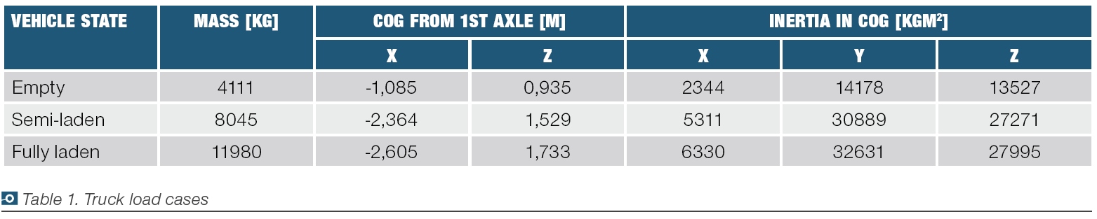
To develop the necessary active steering logic, we used simulations. Simple models built in Matlab Simulink, and validated vehicle models built in SIMPACK [4]. The controller’s environment was based on a real EBS (Electronic Braking System). It worked with 10ms discrete step time and sensors noise content was also measured. But these noises were not filtered in our controllers. The reason is that, the simulated sensors are containing integrated noise filters [5]. Simple Simulink models were used to compare control strategies. These models represented several load cases. The base truck for these was an Iveco Eurocargo ML120E22P [6] – Table 1. In the truck’s used load cases it could be seen that the empty and fully laden truck’s axle loads significantly differ. It is also the case for masses and inertias. The Simulink model’s fundament is a bicycle model – (1) and (2) define the necessary phenomena. Table 3 contains the used notation meanings.
(1) ![]()
(2) 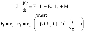
In (2), cornering stiffness is a constant. For this simple model a linearized tire model was used. In this, the 90% of tire normal force was the maximum lateral force, which was reached at 0,08rad lateral slip. Over this slip value no further lateral force increasing was taken. The developed final controller was also tested with validated tractor model. This was based on measurements of an MAN TGA tractor. Another investigation option was tire wear conditions. A new set of truck tires costs more than 4000€, so the owners use the tires as long as it possible. But in case of any other happenings which cause tire grip loss, it is a requirement to ensure the highest safety. We investigated tires with 30% gripping ability.
The Strategies
To figure out which one control strategy is the best, five techniques were investigated:
- PID control, LQ regulation (LQR) and Neuro-Fuzzy approach
- H∞ control
- Adaptive Reference Model (ARM)
With this list we tried to select simple empirical strategies (PID and Neuro-Fuzzy) and some in theoretical ways optimized strategies (LQR and H∞). The fifth strategy (ARM) is working with special solutions which are only valid for this model.
The controller’s aim was to ensure the best reference yaw rate following property. In case of comparisons the control signal was equation (2)’s external control torque – M. This input is acting around the vehicle’s vertical axle. The design was based every time on a semi laden truck’s parameters, which is running with new tires. Reference yaw rate was originated from a semi laden truck model, which’s steering behaviour was neutral. We represent only PID, H∞ and ARM results, because LQR and Neuro-Fuzzy results are very similar to PID.
PID Control
The control signal was only yaw rate difference from the ideal vehicle state. For the tuning of this controller, some physical calculations were made. Redefining (2) to a steady state (yaw rate is constant), left side of (3) is given. From this with the neglecting of steering angles and sideslip angle the right side of (3) could be written. It says that the yaw rate is proportional to the external torque in a steady state case where velocity and cornering stiffness parameters are constants.
(3) ![]()
So, (3) provided a proportional gain value, but that wasn’t enough accurate. To reach a good reference signal following property, another integrator part was needed, and we didn’t use derivative part for this control logic. As it was mentioned increased mass (relative to passenger cars) results in lower vehicle behaviour frequencies, and the steering system has also a relative high latency. Both things show in that way, which is not requesting fast control behaviour.
H∞ control
With this method another approach could be used for controller design: the aim is to hold the measured outputs below a predefined limit [7]. For this also predefined inputs are the excitations, which’s amplitudes are defined, but the carrying frequencies could be theoretically anything from 0 to infinite. The highest singular value of the closed loop system (the controlled system with the controller) will be the H∞ norm [8]. If it’s less than 1, the system is defined as robust. We investigated the number of internal states of the resulted controller (because this method results a full state space controller): Matlab’s hinfsyn command and HIFOO [9] were used. With hinfsyn, a full order controller could be computed. With HIFOO, the order of the controller could be given by the user, or the software searches the lowest order robust controller. In our case (steered wheel angle is the noise input; external torque is the control input; lateral acceleration, yaw rate and control torque are the measured outputs; lateral acceleration and yaw rate are the controller inputs) the HIFOO algorithm found zero order controllers as lowest order controllers (third order is the full order for this state space realization). But without internal state variable the control signal wasn’t smoother like in the previous cases. With 1, 2 or 3 controller states the control signal noise ratio could be decreased. The lowest H∞ norm was reached by 1st order controllers. As it was mentioned, we also investigated the worn tires effects with 30% gripping ability. Our final H∞ controller performs in every case less than 1 as H∞ norm. The conclusion was that the “stronger” controllers were not enough robust in case of worn rear tires – Table 2. As it can be seen the mentioned case is the most dangerous.
.jpg)
Adaptive Reference Model
It is common in the previous control techniques that in every case the control signal is resulted by some difference between the actual and ideal vehicle states, so there is a negative feedback from the controlled signal to the control signal. The control signal decreases the difference between the ideal and actual states, which decreases the control signal’s amplitude. This phenomenon results that only with an integrator part could be good reference signal following property achieved. Our aim was to separate the controller’s input signals from the control signal’s effect – to reach a control loop without a feedback from the controlled signals to the control signal. As it was mentioned, the cornering stiffness parameters in (2) are constants. In the linear zone of the vehicle behaviour they are in reality also approximately constants (which depend on the average road friction only in this case, if the wheel forces are summarized in each axle). With the defined bicycle model ((1) and (2)) equations, it is easy to estimate the cornering stiffness parameters. For this, the bicycle model’s axle sideslip angles must be estimated – with using of a state estimator it is possible. So there are two vehicle trajectories: the first one is resulted by the classical reference model. The second one is resulted by the adaptive reference model. Both are independent from the vehicle’s actual state (controlled or not). With the difference of these reference model’s resulted outputs (4), the necessary control torque could be easily calculated.
(4) ![]()
Comparison Results
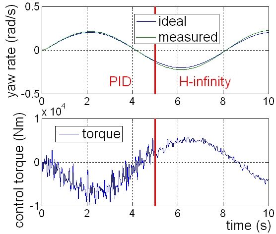
Figure 1: With PID and H∞ strategies controlled vehicles yaw rate
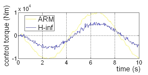
Figure 2: Comparison of H∞ and ARM control signal
For the representation of the control techniques a laden simple vehicle model is chosen, which is light oversteered. As it was mentioned, only the H∞ strategy has an integrated integrator part – the controller’s internal state. This property results much smoother control signal, Figure 1 proves this. It could be also seen, that the H∞ strategy resulted weaker reference signal following property. LQR and Neuro-Fuzzy results aren’t here represented, because they are very similar to PID results. Figure 2 shows the comparison of the H∞ and ARM control signal. The ARM control results stronger control signal (and better reference following, which is not presented because it is very similar also to the PID case), and what is more the control torque is smoother and has smaller phase latency – probably this control strategy lets the driver to feel more direct reaction.
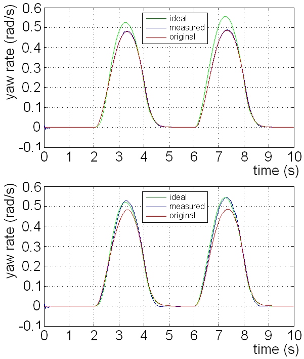
Figure 3: MAN TGA’s uncontrolled and ARM active steering controlled states
In Figure 3’s left the mentioned validated MAN TGA tractor’s uncontrolled state could be seen. There are three signals: ideal, which is resulted by a classical reference model; original, which is estimated by the ARM; measured, which is the vehicle’s measured state. Our aim is to move the measured state from the original to the ideal, and at the same time the estimated ideal and original states should be the same. The result is shown by the right of Figure 3 – the control is done with active front wheel steering. As it can be seen, the reference models estimated states both stayed the same, and the vehicle state moved to the ideal state.
Conclusions
Our aim was to find the best control logic for an active steering control. The logic has to work in case of low frequency excitations – in the high frequency range braking units start to work, which does not allow the steering unit’s accurate control. In theses cases PID controls with state machines are the best choices.
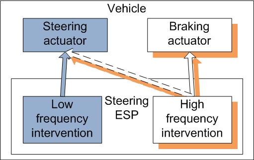
Figure 4.
We compared several techniques with simulation models, but later real measurements are needed. PID, LQR and Neuro-Fuzzy use direct feedback from the controller signal to the control signal – often a simple proportional gain is calculated (even if the gain’s actual value is a lookup table). These techniques result high control signal noise ratio which is not allowed in an active steering system. The H∞ technique contains internal controller states; it is very useful to decrease the control signal’s noise ratio. Another way is used in case of ARM. The developed controller’s efficiency was high enough in the investigated cases. Further tests and investigations are needed to figure out how useful and stable this solution is.
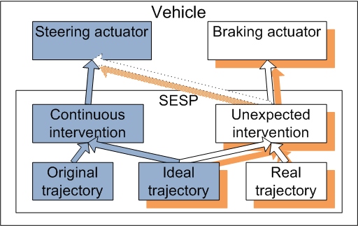
Figure 5.
In the future active steering control will be hopefully available also in commercial vehicle category. Probably the first series of commercial vehicle active steering systems will control only the rear steered axle, if it’s integrated – this solution is already in use, but the used logics not control vehicle stability. The efficiency of this control option is high enough to test several solutions. With the developed ARM an active servo engine control also could be created, which could teach the driver where the vehicle’s actual limits are.
References
[1] E. K. Liebemann, K. Meder, J. Schuch, G. Nenninger: Safety and Performance Enhancement: The Bosch Electronic Stability Control (ESP), 19th International Technical Conference on the Enhanced Safety of Vehicles, June 6-9, 2005, Washington D.C.
[2] Knorr-Bremse GmbH Systeme für Nutzfarzeuge, Product Documentation Site, http://www.knorr-bremsecvs.com/en-gb/documentation/Pages/Documentation.aspx
[3] Hans B. Pacejka: Tyre and Vehicle Dynamics Second Edition, ISBN-10: 0-7506-6918-7, Chapter 1.2.
[4] SIMPACK AG, SIMPACK Multi-Body Simulation Software, http://www.simpack.de
[5] Robert Bosch GmbH, Automotive Sensors – The Bosch Yellow Jackets, 2002, ISBN-13: 978-0-8376-1087-0
[6] Iveco ML120E22P technical data sheet, http://web.iveco.com/uk/collections/technical_sheets/Documents/eurocargo/Eurocargo-120/120E22_truck.pdf
[7] Kemin Zhou, John C. Doyle, Keith Glover: Robust and Optimal Control, Cloth, 1996, ISBN 0-13-456567-3
[8] Bruce A. Francis: A Course in H∞ Control Theory, Springer Verlag, Berlin, Heidelberg, 1987, ISBN 3-540-17069-3
[9] S. Gumussoy, D. Henrion, M. Millstone and M.L. Overton, Multiobjective Robust Control with HIFOO 2.0, Proceedings of the IFAC Symposium on Robust Control Design, Haifa, Israel, 2009
Appendix
.jpg)
Author data
Zoltán Hankovszki: Budapest University of Technology and Economics, Stoczek street 6, J building 5th floor, H-1111, Budapest, Hungary, E-mail: Hankovszki.Zoltan@auto.bme.hu
Roland Kovács: Budapest University of Technology and Economics, Stoczek street 6, J building 5th floor, H-1111, Budapest, Hungary, E-mail: kovacsr@ejjt.bme.hu
Dr. László Palkovics: Budapest University of Technology and Economics, Stoczek street 6, J building 5th floor, H-1111, Budapest, Hungary, E-mail: palko@auto.bme.hu

Ajánló

Autótechnika
- A JÖVÕ MOBILITÁSA ELÕADÁSSOROZAT
- Suttogó fékbetétek: Akusztikai tesztek a fokozott fékezési
- VÁSÁRIDÕ